
Time Based Utilities and Drift Removal
[1]:
%load_ext autoreload
%autoreload 2

import matplotlib.pyplot as plt
import xarray as xr
import numpy as np

from xmip.utils import google_cmip_col
from xmip.preprocessing import combined_preprocessing
[2]:
from dask_gateway import Gateway
g = Gateway()
running_clusters = g.list_clusters()
print(running_clusters)
for c in running_clusters:
    # g.stop_cluster()
    cluster = g.connect(c.name)
    cluster.close()
print(running_clusters)
[]
[]
[3]:
from distributed import Client
from dask_gateway import GatewayCluster
cluster = GatewayCluster()
cluster.scale(30)
cluster
[4]:
client = Client(cluster)
client
[4]:
Client
|
Cluster
|
Loading example data
[5]:
zkwargs = {'consolidated':True, 'use_cftime':True}
kwargs = {'zarr_kwargs':zkwargs, 'preprocess':combined_preprocessing, 'aggregate':False}

col = google_cmip_col()


cat = col.search(source_id='CanESM5-CanOE', variable_id='thetao')


ddict_historical = cat.search(experiment_id='historical').to_dataset_dict(**kwargs)
ddict_ssp585 = cat.search(experiment_id='ssp585').to_dataset_dict(**kwargs)
ddict_picontrol = cat.search(experiment_id='piControl').to_dataset_dict(**kwargs)
--> The keys in the returned dictionary of datasets are constructed as follows:
        'activity_id.institution_id.source_id.experiment_id.member_id.table_id.variable_id.grid_label.zstore.dcpp_init_year.version'
--> The keys in the returned dictionary of datasets are constructed as follows:
        'activity_id.institution_id.source_id.experiment_id.member_id.table_id.variable_id.grid_label.zstore.dcpp_init_year.version'
--> The keys in the returned dictionary of datasets are constructed as follows:
        'activity_id.institution_id.source_id.experiment_id.member_id.table_id.variable_id.grid_label.zstore.dcpp_init_year.version'
Pick some example data
Lets pick a particular member and define a point in x/y/z space that we will use throughout this demonstration to extract timeseries at the same point.
[6]:
ds_control = ddict_picontrol['CMIP.CCCma.CanESM5-CanOE.piControl.r1i1p2f1.Omon.thetao.gn.gs://cmip6/CMIP6/CMIP/CCCma/CanESM5-CanOE/piControl/r1i1p2f1/Omon/thetao/gn/v20190429/.nan.20190429']
ds_historical = ddict_historical['CMIP.CCCma.CanESM5-CanOE.historical.r1i1p2f1.Omon.thetao.gn.gs://cmip6/CMIP6/CMIP/CCCma/CanESM5-CanOE/historical/r1i1p2f1/Omon/thetao/gn/v20190429/.nan.20190429']
ds_ssp585 = ddict_ssp585['ScenarioMIP.CCCma.CanESM5-CanOE.ssp585.r1i1p2f1.Omon.thetao.gn.gs://cmip6/CMIP6/ScenarioMIP/CCCma/CanESM5-CanOE/ssp585/r1i1p2f1/Omon/thetao/gn/v20190429/.nan.20190429']

# Pick a random location in x/y/z space to use as an exmple
roi = {'x':100,'y':220, 'lev':30}
Visulalizing branching from the control run
Lets first start by visualizing the example point of our data
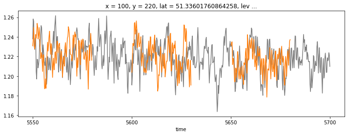
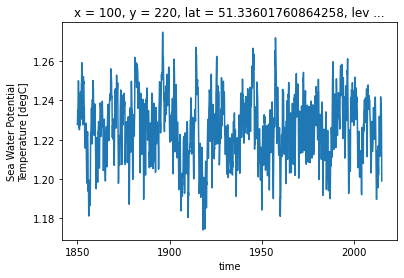
[7]:
# ok lets just plot them together
ds_control.isel(**roi).thetao.plot(color='0.5')
ds_historical.isel(**roi).thetao.plot(color='C1')
[7]:
[<matplotlib.lines.Line2D at 0x7f98efd3cfa0>]
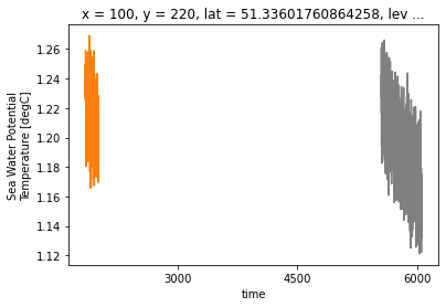
Hmm well that doesnt look good. Its because the control run follows a different time convention. But we can check when the run was branched out exactly by looking at the metadata of the historical run:
[8]:
{k:v for k,v in ds_historical.attrs.items() if 'parent' in k}
[8]:
{'CCCma_parent_runid': 'canoecpl-007',
 'YMDH_branch_time_in_parent': '5550:01:01:00',
 'branch_time_in_parent': 1350500.0,
 'parent_activity_id': 'CMIP',
 'parent_experiment_id': 'piControl',
 'parent_mip_era': 'CMIP6',
 'parent_source_id': 'CanESM5-CanOE',
 'parent_time_units': 'days since 1850-01-01 0:0:0.0',
 'parent_variant_label': 'r1i1p2f1'}
And of course there is a tool in here that makes translating these a bit easier. We can just convert time conventions from child to parent or vice versa.
[9]:
from xmip.drift_removal import unify_time

# the default will adjust the time convention from the first input (`parent`) to the second (`child`)
ds_control_adj, ds_historical_adj = unify_time(ds_control, ds_historical)
[10]:
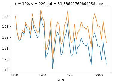
# ok lets just plot them together
ds_control_adj.isel(**roi).thetao.plot(color='0.5')
ds_historical_adj.isel(**roi).thetao.plot(color='C1')
[10]:
[<matplotlib.lines.Line2D at 0x7f98ee01f490>]
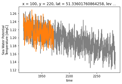
That looks more sensible, but with all the wiggles its a bit tough to see. Since this run seems to be branched of at the first time step of the control ouput (the run is probably much longer, but not all data was provided to the archive), lets just cut to the first couple of timesteps to check in more detail.
[11]:
# ok lets just plot them together
ds_control_adj.isel(**roi, time=slice(0,24)).thetao.plot()
ds_historical_adj.isel(**roi, time=slice(0,24)).thetao.plot()
[11]:
[<matplotlib.lines.Line2D at 0x7f98bfc65910>]
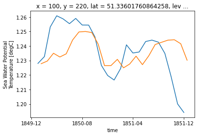
That looks pretty good, but the values are slightly shifted. This is due to the fact that for the ‘untouched’ CMIP6 monthly data uses a timestamp in the ‘middle’ of the month, whereas our adustment uses the start of the month. We can quickly adjust that:
[12]:
from xmip.drift_removal import replace_time
# with the defaults it will just replace the dates with new ones which have time stamps at the beginning of the month.
ds_historical_adj = replace_time(ds_historical_adj)
[13]:
# ok lets just plot them together again
ds_control_adj.isel(**roi, time=slice(0,24)).thetao.plot()
ds_historical_adj.isel(**roi, time=slice(0,24)).thetao.plot()
[13]:
[<matplotlib.lines.Line2D at 0x7f98bfce4b20>]
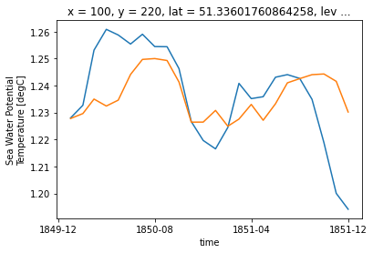
BINGO
OK now lets look at all the members:
[14]:
for name, ds in ddict_historical.items():
    print(name, ds.attrs['branch_time_in_parent'])
CMIP.CCCma.CanESM5-CanOE.historical.r2i1p2f1.Omon.thetao.gn.gs://cmip6/CMIP6/CMIP/CCCma/CanESM5-CanOE/historical/r2i1p2f1/Omon/thetao/gn/v20190429/.nan.20190429 1368750.0
CMIP.CCCma.CanESM5-CanOE.historical.r3i1p2f1.Omon.thetao.gn.gs://cmip6/CMIP6/CMIP/CCCma/CanESM5-CanOE/historical/r3i1p2f1/Omon/thetao/gn/v20190429/.nan.20190429 1387000.0
CMIP.CCCma.CanESM5-CanOE.historical.r1i1p2f1.Omon.thetao.gn.gs://cmip6/CMIP6/CMIP/CCCma/CanESM5-CanOE/historical/r1i1p2f1/Omon/thetao/gn/v20190429/.nan.20190429 1350500.0
Hmmm, these were all branched out at a different time! This is actually quite common, but it means to visualize these we will have to convert the time into the conventions of the parent (control) run. Thats pretty easy though!
[16]:
# replace the timestamp with the first of the month for the control run and plot
# we will also average the data yearly to remove some of the visual noise

plt.figure(figsize=[12,4])
replace_time(ds_control).isel(**roi).thetao.coarsen(time=3).mean().isel(time=slice(0,150*4)).plot(color='0.5')

# now we loop through all the historical members, adjust the time and plot them in the same way,
# but only for the first 20 years
for name, ds in ddict_historical.items():
    _, ds_adj = unify_time(ds_control, ds, adjust_to='parent')
    ds_adj.isel(**roi).thetao.coarsen(time=3).mean().isel(time=slice(0,30*4)).plot(color='C1')
You can see that all the ‘connection points’ seem to match up!
Removing control drift
This was a neat exercise, but you might have noticed that the control run shows a pretty pronounced trend (decreasing temperature). Since this is an unforced control run, we have to assume that the model is not completely equilibrated and continues to drift. This drift can affect the runs which are branched off this run.
It is often desirable to remove the drift, or more precisely subtract the linear trend of the control run over the time period of the branched off runs. xmip makes this easy.
In this context the words trend and drift are used as follows: - trend general expression for a linear trend over a timeseries - drift particularly the control run trend
Rechunking the control run
Since most CMIP6 datasets are chunked into pretty small time chunks, applying any operation along the time axis is very difficult to do with dask. Lets use the rechunker package to write a temporary dataset that is chunked in space, not time.
We will save this (large) dataset in the Pangeo scratch bucket
[19]:
# setting up the scratch bucket
import os
import fsspec
PANGEO_SCRATCH = os.environ['PANGEO_SCRATCH']+'cmip6_pp_demo'
path = f'{PANGEO_SCRATCH}/test_rechunked.zarr'
temp_path = f'{PANGEO_SCRATCH}/test_rechunked_temp.zarr'
mapper = fsspec.get_mapper(path)
mapper_temp = fsspec.get_mapper(temp_path)
[20]:
if not mapper.fs.exists(path):
    # recompute the rechunked data into the scratch bucket (is only triggered when the temporary store was erased)

    # Remove the temp store if for some reason that still exists
    if mapper.fs.exists(temp_path):
        mapper.fs.rm(temp_path, recursive=True)
    from rechunker import rechunk
    target_chunks = {
        'thetao': {'time':6012, 'lev':1, 'x':3, 'y':291},
        'x': {'x':3},
        'y': {'y':291},
        'lat': {'x':3, 'y':291},
        'lev': {'lev':1},
        'lon': {'x':3, 'y':291},
        'time': {'time':6012},
    }
    max_mem = '1GB'

    array_plan = rechunk(ds_control[['thetao']], target_chunks, max_mem, mapper, temp_store=mapper_temp)
    array_plan.execute(retries=10)

ds_control_rechunked = xr.open_zarr(mapper, use_cftime=True)
ds_control_rechunked
[20]:
<xarray.Dataset>
Dimensions:  (lev: 45, time: 6012, x: 360, y: 291)
Coordinates:
    lat      (y, x) float64 dask.array<chunksize=(291, 3), meta=np.ndarray>
  * lev      (lev) float64 3.047 9.454 16.36 ... 5.126e+03 5.375e+03 5.625e+03
    lon      (y, x) float64 dask.array<chunksize=(291, 3), meta=np.ndarray>
  * time     (time) object 5550-01-16 12:00:00 ... 6050-12-16 12:00:00
  * x        (x) int32 0 1 2 3 4 5 6 7 8 ... 351 352 353 354 355 356 357 358 359
  * y        (y) int32 0 1 2 3 4 5 6 7 8 ... 282 283 284 285 286 287 288 289 290
Data variables:
    thetao   (time, lev, y, x) float32 dask.array<chunksize=(6012, 1, 291, 3), meta=np.ndarray>
Attributes: (12/58)
    CCCma_model_hash:            932b659de600c6a0e94f619abaf9cc79eabcd337
    CCCma_parent_runid:          canoecpl-007
    CCCma_pycmor_hash:           3ecdc18eb7c1f7fbce0346850f41adf815d9fb66
    CCCma_runid:                 c2-pictrl
    Conventions:                 CF-1.7 CMIP-6.2
    YMDH_branch_time_in_child:   5550:01:01:00
    ...                          ...
    title:                       CanESM5-CanOE output prepared for CMIP6
    tracking_id:                 hdl:21.14100/8b3a90ee-6bf3-496a-ba59-648dded...
    variable_id:                 thetao
    variant_label:               r1i1p2f1
    version:                     v20190429
version_id: v20190429- lev: 45
- time: 6012
- x: 360
- y: 291
- lat(y, x)float64dask.array<chunksize=(291, 3), meta=np.ndarray>
- bounds :
- vertices_latitude
- long_name :
- latitude
- standard_name :
- latitude
- units :
- degrees_north
Array Chunk Bytes 818.44 kiB 6.82 kiB Shape (291, 360) (291, 3) Count 121 Tasks 120 Chunks Type float64 numpy.ndarray - lev(lev)float643.047 9.454 ... 5.375e+03 5.625e+03
- axis :
- Z
- bounds :
- lev_bnds
- long_name :
- ocean depth coordinate
- positive :
- down
- standard_name :
- depth
- units :
- m
array([3.046773e+00, 9.454049e+00, 1.636397e+01, 2.389871e+01, 3.220929e+01, 4.148185e+01, 5.194513e+01, 6.387905e+01, 7.762451e+01, 9.359412e+01, 1.122835e+02, 1.342823e+02, 1.602840e+02, 1.910925e+02, 2.276233e+02, 2.708962e+02, 3.220169e+02, 3.821444e+02, 4.524429e+02, 5.340197e+02, 6.278525e+02, 7.347150e+02, 8.551112e+02, 9.892289e+02, 1.136922e+03, 1.297724e+03, 1.470893e+03, 1.655472e+03, 1.850365e+03, 2.054414e+03, 2.266454e+03, 2.485371e+03, 2.710133e+03, 2.939812e+03, 3.173588e+03, 3.410756e+03, 3.650712e+03, 3.892950e+03, 4.137047e+03, 4.382654e+03, 4.629485e+03, 4.877303e+03, 5.125919e+03, 5.375177e+03, 5.624952e+03]) - lon(y, x)float64dask.array<chunksize=(291, 3), meta=np.ndarray>
- bounds :
- vertices_longitude
- long_name :
- longitude
- standard_name :
- longitude
- units :
- degrees_east
Array Chunk Bytes 818.44 kiB 6.82 kiB Shape (291, 360) (291, 3) Count 121 Tasks 120 Chunks Type float64 numpy.ndarray - time(time)object5550-01-16 12:00:00 ... 6050-12-...
- axis :
- T
- bounds :
- time_bnds
- long_name :
- time
- standard_name :
- time
array([cftime.DatetimeNoLeap(5550, 1, 16, 12, 0, 0, 0), cftime.DatetimeNoLeap(5550, 2, 15, 0, 0, 0, 0), cftime.DatetimeNoLeap(5550, 3, 16, 12, 0, 0, 0), ..., cftime.DatetimeNoLeap(6050, 10, 16, 12, 0, 0, 0), cftime.DatetimeNoLeap(6050, 11, 16, 0, 0, 0, 0), cftime.DatetimeNoLeap(6050, 12, 16, 12, 0, 0, 0)], dtype=object) - x(x)int320 1 2 3 4 5 ... 355 356 357 358 359
- long_name :
- cell index along first dimension
- units :
- 1
array([ 0, 1, 2, ..., 357, 358, 359], dtype=int32)
- y(y)int320 1 2 3 4 5 ... 286 287 288 289 290
- long_name :
- cell index along second dimension
- units :
- 1
array([ 0, 1, 2, ..., 288, 289, 290], dtype=int32)
- thetao(time, lev, y, x)float32dask.array<chunksize=(6012, 1, 291, 3), meta=np.ndarray>
- cell_measures :
- area: areacello volume: volcello
- cell_methods :
- area: mean where sea time: mean
- comment :
- Diagnostic should be contributed even for models using conservative temperature as prognostic field.
- coordinates :
- latitude longitude
- long_name :
- Sea Water Potential Temperature
- original_name :
- votemper
- standard_name :
- sea_water_potential_temperature
- units :
- degC
Array Chunk Bytes 105.58 GiB 20.02 MiB Shape (6012, 45, 291, 360) (6012, 1, 291, 3) Count 5401 Tasks 5400 Chunks Type float32 numpy.ndarray
- CCCma_model_hash :
- 932b659de600c6a0e94f619abaf9cc79eabcd337
- CCCma_parent_runid :
- canoecpl-007
- CCCma_pycmor_hash :
- 3ecdc18eb7c1f7fbce0346850f41adf815d9fb66
- CCCma_runid :
- c2-pictrl
- Conventions :
- CF-1.7 CMIP-6.2
- YMDH_branch_time_in_child :
- 5550:01:01:00
- YMDH_branch_time_in_parent :
- 5550:01:01:00
- activity_id :
- CMIP
- branch_method :
- Spin-up documentation
- branch_time_in_child :
- 1350500.0
- branch_time_in_parent :
- 1350500.0
- cmor_version :
- 3.5.0
- contact :
- ec.cccma.info-info.ccmac.ec@canada.ca
- creation_date :
- 2019-12-11T20:58:53Z
- data_specs_version :
- 01.00.31
- experiment :
- pre-industrial control
- experiment_id :
- piControl
- external_variables :
- areacello volcello
- forcing_index :
- 1
- frequency :
- mon
- further_info_url :
- https://furtherinfo.es-doc.org/CMIP6.CCCma.CanESM5-CanOE.piControl.none.r1i1p2f1
- grid :
- ORCA1 tripolar grid, 1 deg with refinement to 1/3 deg within 20 degrees of the equator; 361 x 290 longitude/latitude; 45 vertical levels; top grid cell 0-6.19 m
- grid_label :
- gn
- history :
- 2019-12-11T20:58:53Z ;rewrote data to be consistent with CMIP for variable thetao found in table Omon.
- initialization_index :
- 1
- institution :
- Canadian Centre for Climate Modelling and Analysis, Environment and Climate Change Canada, Victoria, BC V8P 5C2, Canada
- institution_id :
- CCCma
- intake_esm_dataset_key :
- CMIP.CCCma.CanESM5-CanOE.piControl.r1i1p2f1.Omon.thetao.gn.gs://cmip6/CMIP6/CMIP/CCCma/CanESM5-CanOE/piControl/r1i1p2f1/Omon/thetao/gn/v20190429/.nan.20190429
- intake_esm_varname :
- None
- license :
- CMIP6 model data produced by The Government of Canada (Canadian Centre for Climate Modelling and Analysis, Environment and Climate Change Canada) is licensed under a Creative Commons Attribution ShareAlike 4.0 International License (https://creativecommons.org/licenses). Consult https://pcmdi.llnl.gov/CMIP6/TermsOfUse for terms of use governing CMIP6 output, including citation requirements and proper acknowledgment. Further information about this data, including some limitations, can be found via the further_info_url (recorded as a global attribute in this file) and at https:///pcmdi.llnl.gov/. The data producers and data providers make no warranty, either express or implied, including, but not limited to, warranties of merchantability and fitness for a particular purpose. All liabilities arising from the supply of the information (including any liability arising in negligence) are excluded to the fullest extent permitted by law.
- mip_era :
- CMIP6
- netcdf_tracking_ids :
- hdl:21.14100/8b3a90ee-6bf3-496a-ba59-648ddedb007c hdl:21.14100/d73e30c1-ade5-4187-9276-a765675ba594 hdl:21.14100/e8ec6a5c-1b1e-4f38-bb6c-3cf749331a72 hdl:21.14100/f40c6071-ebbe-4c39-9552-fb9d44cf18c2 hdl:21.14100/8e9cdeca-d27d-4f5d-9294-ae2017eda51e hdl:21.14100/6bfc80cc-b651-4749-add2-47230f00b4f7 hdl:21.14100/3838dd2c-9838-4cee-8057-420a285c16b7 hdl:21.14100/6a8df388-8eaf-42db-9a8c-fb785f00553a hdl:21.14100/94d17f37-bc9c-4a71-b311-701afe5002db hdl:21.14100/ce804047-111e-4140-b7e4-aaabe712baeb hdl:21.14100/c46a5aff-afca-40e3-a41f-2b4837f8da7a hdl:21.14100/f3c29ca2-63f3-4c66-970e-202a98287e76 hdl:21.14100/44a989f3-55e7-40ac-bcd6-a322ad98a8a4 hdl:21.14100/2fa7efbf-b263-47fa-b085-15024d22a9b2 hdl:21.14100/9189ae2c-157c-4b2e-a143-f00196de2b15 hdl:21.14100/881d762f-8479-4a2e-9b24-7d6724411d7a hdl:21.14100/7d5a15c7-bd57-4d60-9377-6cb8ce5544d8 hdl:21.14100/c8b6c648-a238-4520-b8d0-984c18584737 hdl:21.14100/5fa556fb-d772-4d65-99fd-7ee524df4669 hdl:21.14100/5f5a48d9-8d6f-44f8-8854-7f7d168fa95b hdl:21.14100/0e13a49d-446a-426e-af98-5d068921ac80 hdl:21.14100/50ac7e17-f501-409e-bb78-a3a844203c3d hdl:21.14100/d9e74964-17d1-46b4-ae37-c85da9673408 hdl:21.14100/46e16c1b-edcc-4353-ae2a-a0a661cb68e5 hdl:21.14100/9ce4dc44-eaca-4b98-a999-347d28808a5b hdl:21.14100/a38c0f47-4f5d-4541-8acf-882f7fef6c4e hdl:21.14100/8198bd12-1e6a-4d8c-a0a6-03e085943d4d hdl:21.14100/6f5b0e9a-b79d-4321-9a86-1d68c58559ae hdl:21.14100/24e2daea-7556-46c8-9e08-c1109e212910 hdl:21.14100/ce7aafab-46b3-4ec2-9abb-4b107179a021 hdl:21.14100/40b76661-3806-40bf-9381-20a1918c2acd hdl:21.14100/99cb0d3d-bc7d-4469-b232-c3529a9f45cc hdl:21.14100/6c6f53e7-b15f-4382-b1e5-07354bae1aa9 hdl:21.14100/7c2657e6-ccf3-48ae-9f4b-a46a85b4ce9c hdl:21.14100/f1b55d85-0633-44e9-b1cf-8f55241ddf44 hdl:21.14100/0c6fda9b-3959-49c4-af27-65340573c503 hdl:21.14100/8c5acf30-cc61-44ee-a496-c2f8e8258270 hdl:21.14100/f4b44462-d3d7-4932-90c4-34d9a8f726de hdl:21.14100/d5425f68-8ad5-4fec-8309-3a79eb3195e5 hdl:21.14100/e0cb2937-21ce-4277-8927-361db0d7f96c hdl:21.14100/682a5332-b6ef-4044-ae4f-e692cb30b61f hdl:21.14100/2744f541-25e1-485f-8e7a-a54dbb9b35f6 hdl:21.14100/b3a492e0-ea86-49fb-98b3-5c20c5c09d5e hdl:21.14100/6897611a-8205-4a6a-9e2b-d15153a3b238 hdl:21.14100/b92451d5-66e7-4477-9bbe-5b0938ff537c hdl:21.14100/14c3e40f-46c0-4236-b632-c50b741c9865 hdl:21.14100/712e0694-fd3e-47de-95ec-f8758f4f427e hdl:21.14100/09026096-df9c-44b5-a3be-38d7859ae189 hdl:21.14100/05345fcc-3261-47e4-81b4-24caeb0674bc hdl:21.14100/9a3ea32e-84bb-4d7a-a11f-6c560915efa4
- nominal_resolution :
- 100 km
- parent_activity_id :
- CMIP
- parent_experiment_id :
- piControl-spinup
- parent_mip_era :
- CMIP6
- parent_source_id :
- CanESM5-CanOE
- parent_time_units :
- days since 1850-01-01 0:0:0.0
- parent_variant_label :
- r1i1p2f1
- physics_index :
- 2
- product :
- model-output
- realization_index :
- 1
- realm :
- ocean
- references :
- Geoscientific Model Development Special issue on CanESM5 (https://www.geosci-model-dev.net/special_issue989.html)
- source :
- CanESM5-CanOE (2019): aerosol: interactive atmos: CanAM5 (T63L49 native atmosphere, T63 Linear Gaussian Grid; 128 x 64 longitude/latitude; 49 levels; top level 1 hPa) atmosChem: specified oxidants for aerosols land: CLASS3.6/CTEM1.2 landIce: specified ice sheets ocean: NEMO3.4.1 (ORCA1 tripolar grid, 1 deg with refinement to 1/3 deg within 20 degrees of the equator; 361 x 290 longitude/latitude; 45 vertical levels; top grid cell 0-6.19 m) ocnBgchem: Canadian Ocean Ecosystem (CanOE) with OMIP prescribed carbon chemistry seaIce: LIM2
- source_id :
- CanESM5-CanOE
- source_type :
- AOGCM
- status :
- 2020-12-31;created; by gcs.cmip6.ldeo@gmail.com
- sub_experiment :
- none
- sub_experiment_id :
- none
- table_id :
- Omon
- table_info :
- Creation Date:(24 July 2019) MD5:c93735846d66458966fc81f390b2d714
- title :
- CanESM5-CanOE output prepared for CMIP6
- tracking_id :
- hdl:21.14100/8b3a90ee-6bf3-496a-ba59-648ddedb007c hdl:21.14100/d73e30c1-ade5-4187-9276-a765675ba594 hdl:21.14100/e8ec6a5c-1b1e-4f38-bb6c-3cf749331a72 hdl:21.14100/f40c6071-ebbe-4c39-9552-fb9d44cf18c2 hdl:21.14100/8e9cdeca-d27d-4f5d-9294-ae2017eda51e hdl:21.14100/6bfc80cc-b651-4749-add2-47230f00b4f7 hdl:21.14100/3838dd2c-9838-4cee-8057-420a285c16b7 hdl:21.14100/6a8df388-8eaf-42db-9a8c-fb785f00553a hdl:21.14100/94d17f37-bc9c-4a71-b311-701afe5002db hdl:21.14100/ce804047-111e-4140-b7e4-aaabe712baeb hdl:21.14100/c46a5aff-afca-40e3-a41f-2b4837f8da7a hdl:21.14100/f3c29ca2-63f3-4c66-970e-202a98287e76 hdl:21.14100/44a989f3-55e7-40ac-bcd6-a322ad98a8a4 hdl:21.14100/2fa7efbf-b263-47fa-b085-15024d22a9b2 hdl:21.14100/9189ae2c-157c-4b2e-a143-f00196de2b15 hdl:21.14100/881d762f-8479-4a2e-9b24-7d6724411d7a hdl:21.14100/7d5a15c7-bd57-4d60-9377-6cb8ce5544d8 hdl:21.14100/c8b6c648-a238-4520-b8d0-984c18584737 hdl:21.14100/5fa556fb-d772-4d65-99fd-7ee524df4669 hdl:21.14100/5f5a48d9-8d6f-44f8-8854-7f7d168fa95b hdl:21.14100/0e13a49d-446a-426e-af98-5d068921ac80 hdl:21.14100/50ac7e17-f501-409e-bb78-a3a844203c3d hdl:21.14100/d9e74964-17d1-46b4-ae37-c85da9673408 hdl:21.14100/46e16c1b-edcc-4353-ae2a-a0a661cb68e5 hdl:21.14100/9ce4dc44-eaca-4b98-a999-347d28808a5b hdl:21.14100/a38c0f47-4f5d-4541-8acf-882f7fef6c4e hdl:21.14100/8198bd12-1e6a-4d8c-a0a6-03e085943d4d hdl:21.14100/6f5b0e9a-b79d-4321-9a86-1d68c58559ae hdl:21.14100/24e2daea-7556-46c8-9e08-c1109e212910 hdl:21.14100/ce7aafab-46b3-4ec2-9abb-4b107179a021 hdl:21.14100/40b76661-3806-40bf-9381-20a1918c2acd hdl:21.14100/99cb0d3d-bc7d-4469-b232-c3529a9f45cc hdl:21.14100/6c6f53e7-b15f-4382-b1e5-07354bae1aa9 hdl:21.14100/7c2657e6-ccf3-48ae-9f4b-a46a85b4ce9c hdl:21.14100/f1b55d85-0633-44e9-b1cf-8f55241ddf44 hdl:21.14100/0c6fda9b-3959-49c4-af27-65340573c503 hdl:21.14100/8c5acf30-cc61-44ee-a496-c2f8e8258270 hdl:21.14100/f4b44462-d3d7-4932-90c4-34d9a8f726de hdl:21.14100/d5425f68-8ad5-4fec-8309-3a79eb3195e5 hdl:21.14100/e0cb2937-21ce-4277-8927-361db0d7f96c hdl:21.14100/682a5332-b6ef-4044-ae4f-e692cb30b61f hdl:21.14100/2744f541-25e1-485f-8e7a-a54dbb9b35f6 hdl:21.14100/b3a492e0-ea86-49fb-98b3-5c20c5c09d5e hdl:21.14100/6897611a-8205-4a6a-9e2b-d15153a3b238 hdl:21.14100/b92451d5-66e7-4477-9bbe-5b0938ff537c hdl:21.14100/14c3e40f-46c0-4236-b632-c50b741c9865 hdl:21.14100/712e0694-fd3e-47de-95ec-f8758f4f427e hdl:21.14100/09026096-df9c-44b5-a3be-38d7859ae189 hdl:21.14100/05345fcc-3261-47e4-81b4-24caeb0674bc hdl:21.14100/9a3ea32e-84bb-4d7a-a11f-6c560915efa4
- variable_id :
- thetao
- variant_label :
- r1i1p2f1
- version :
- v20190429
- version_id :
- v20190429
Calculating the drift over the control run
[21]:
from xmip.drift_removal import calculate_drift, remove_trend
[22]:
drift = calculate_drift(ds_control_rechunked, ds_historical, 'thetao')
drift = drift.load() # This takes a bit, but it is worth loading this small output to avoid repeated computation
drift
/srv/conda/envs/notebook/lib/python3.8/site-packages/xarrayutils/utils.py:85: FutureWarning: ``output_sizes`` should be given in the ``dask_gufunc_kwargs`` parameter. It will be removed as direct parameter in a future version.
  stats = xr.apply_ufunc(
[22]:
<xarray.Dataset>
Dimensions:           (bnds: 2, lev: 45, x: 360, y: 291)
Coordinates:
  * lev               (lev) float64 3.047 9.454 16.36 ... 5.375e+03 5.625e+03
  * x                 (x) int32 0 1 2 3 4 5 6 7 ... 353 354 355 356 357 358 359
  * y                 (y) int32 0 1 2 3 4 5 6 7 ... 284 285 286 287 288 289 290
    trend_time_range  (bnds) <U19 '5550-01-16 12:00:00' '5799-12-16 12:00:00'
Dimensions without coordinates: bnds
Data variables:
    thetao            (lev, y, x) float32 nan nan nan nan ... nan nan nan nan
Attributes: (12/58)
    CCCma_model_hash:            932b659de600c6a0e94f619abaf9cc79eabcd337
    CCCma_parent_runid:          canoecpl-007
    CCCma_pycmor_hash:           3ecdc18eb7c1f7fbce0346850f41adf815d9fb66
    CCCma_runid:                 c2-his01
    Conventions:                 CF-1.7 CMIP-6.2
    YMDH_branch_time_in_child:   1850:01:01:00
    ...                          ...
    variant_label:               r1i1p2f1
    version:                     v20190429
    netcdf_tracking_ids:         hdl:21.14100/05f0fb20-3395-4112-af53-d1b9241...
    version_id:                  v20190429
    intake_esm_varname:          None
intake_esm_dataset_key: CMIP.CCCma.CanESM5-CanOE.historical.r1i1p2f1...- bnds: 2
- lev: 45
- x: 360
- y: 291
- lev(lev)float643.047 9.454 ... 5.375e+03 5.625e+03
- axis :
- Z
- bounds :
- lev_bnds
- long_name :
- ocean depth coordinate
- positive :
- down
- standard_name :
- depth
- units :
- m
array([3.046773e+00, 9.454049e+00, 1.636397e+01, 2.389871e+01, 3.220929e+01, 4.148185e+01, 5.194513e+01, 6.387905e+01, 7.762451e+01, 9.359412e+01, 1.122835e+02, 1.342823e+02, 1.602840e+02, 1.910925e+02, 2.276233e+02, 2.708962e+02, 3.220169e+02, 3.821444e+02, 4.524429e+02, 5.340197e+02, 6.278525e+02, 7.347150e+02, 8.551112e+02, 9.892289e+02, 1.136922e+03, 1.297724e+03, 1.470893e+03, 1.655472e+03, 1.850365e+03, 2.054414e+03, 2.266454e+03, 2.485371e+03, 2.710133e+03, 2.939812e+03, 3.173588e+03, 3.410756e+03, 3.650712e+03, 3.892950e+03, 4.137047e+03, 4.382654e+03, 4.629485e+03, 4.877303e+03, 5.125919e+03, 5.375177e+03, 5.624952e+03]) - x(x)int320 1 2 3 4 5 ... 355 356 357 358 359
- long_name :
- cell index along first dimension
- units :
- 1
array([ 0, 1, 2, ..., 357, 358, 359], dtype=int32)
- y(y)int320 1 2 3 4 5 ... 286 287 288 289 290
- long_name :
- cell index along second dimension
- units :
- 1
array([ 0, 1, 2, ..., 288, 289, 290], dtype=int32)
- trend_time_range(bnds)<U19'5550-01-16 12:00:00' '5799-12-1...
- axis :
- T
- bounds :
- time_bnds
- long_name :
- regression_time_in_reference_run
- standard_name :
- regression_time_bounds
array(['5550-01-16 12:00:00', '5799-12-16 12:00:00'], dtype='<U19')
- thetao(lev, y, x)float32nan nan nan nan ... nan nan nan nan
array([[[nan, nan, nan, ..., nan, nan, nan],
        [nan, nan, nan, ..., nan, nan, nan],
        [nan, nan, nan, ..., nan, nan, nan],
        ...,
        [nan, nan, nan, ..., nan, nan, nan],
        [nan, nan, nan, ..., nan, nan, nan],
        [nan, nan, nan, ..., nan, nan, nan]],

       [[nan, nan, nan, ..., nan, nan, nan],
        [nan, nan, nan, ..., nan, nan, nan],
        [nan, nan, nan, ..., nan, nan, nan],
        ...,
        [nan, nan, nan, ..., nan, nan, nan],
        [nan, nan, nan, ..., nan, nan, nan],
        [nan, nan, nan, ..., nan, nan, nan]],

       [[nan, nan, nan, ..., nan, nan, nan],
        [nan, nan, nan, ..., nan, nan, nan],
        [nan, nan, nan, ..., nan, nan, nan],
        ...,
...
        ...,
        [nan, nan, nan, ..., nan, nan, nan],
        [nan, nan, nan, ..., nan, nan, nan],
        [nan, nan, nan, ..., nan, nan, nan]],

       [[nan, nan, nan, ..., nan, nan, nan],
        [nan, nan, nan, ..., nan, nan, nan],
        [nan, nan, nan, ..., nan, nan, nan],
        ...,
        [nan, nan, nan, ..., nan, nan, nan],
        [nan, nan, nan, ..., nan, nan, nan],
        [nan, nan, nan, ..., nan, nan, nan]],

       [[nan, nan, nan, ..., nan, nan, nan],
        [nan, nan, nan, ..., nan, nan, nan],
        [nan, nan, nan, ..., nan, nan, nan],
        ...,
        [nan, nan, nan, ..., nan, nan, nan],
        [nan, nan, nan, ..., nan, nan, nan],
        [nan, nan, nan, ..., nan, nan, nan]]], dtype=float32)
- CCCma_model_hash :
- 932b659de600c6a0e94f619abaf9cc79eabcd337
- CCCma_parent_runid :
- canoecpl-007
- CCCma_pycmor_hash :
- 3ecdc18eb7c1f7fbce0346850f41adf815d9fb66
- CCCma_runid :
- c2-his01
- Conventions :
- CF-1.7 CMIP-6.2
- YMDH_branch_time_in_child :
- 1850:01:01:00
- YMDH_branch_time_in_parent :
- 5550:01:01:00
- activity_id :
- CMIP
- branch_method :
- Spin-up documentation
- branch_time_in_child :
- 0.0
- branch_time_in_parent :
- 1350500.0
- cmor_version :
- 3.5.0
- contact :
- ec.cccma.info-info.ccmac.ec@canada.ca
- creation_date :
- 2019-12-11T19:02:54Z
- data_specs_version :
- 01.00.31
- experiment :
- all-forcing simulation of the recent past
- experiment_id :
- historical
- external_variables :
- areacello volcello
- forcing_index :
- 1
- frequency :
- mon
- further_info_url :
- https://furtherinfo.es-doc.org/CMIP6.CCCma.CanESM5-CanOE.historical.none.r1i1p2f1
- grid :
- ORCA1 tripolar grid, 1 deg with refinement to 1/3 deg within 20 degrees of the equator; 361 x 290 longitude/latitude; 45 vertical levels; top grid cell 0-6.19 m
- grid_label :
- gn
- history :
- 2019-12-11T19:02:54Z ;rewrote data to be consistent with CMIP for variable thetao found in table Omon.
- initialization_index :
- 1
- institution :
- Canadian Centre for Climate Modelling and Analysis, Environment and Climate Change Canada, Victoria, BC V8P 5C2, Canada
- institution_id :
- CCCma
- license :
- CMIP6 model data produced by The Government of Canada (Canadian Centre for Climate Modelling and Analysis, Environment and Climate Change Canada) is licensed under a Creative Commons Attribution ShareAlike 4.0 International License (https://creativecommons.org/licenses). Consult https://pcmdi.llnl.gov/CMIP6/TermsOfUse for terms of use governing CMIP6 output, including citation requirements and proper acknowledgment. Further information about this data, including some limitations, can be found via the further_info_url (recorded as a global attribute in this file) and at https:///pcmdi.llnl.gov/. The data producers and data providers make no warranty, either express or implied, including, but not limited to, warranties of merchantability and fitness for a particular purpose. All liabilities arising from the supply of the information (including any liability arising in negligence) are excluded to the fullest extent permitted by law.
- mip_era :
- CMIP6
- nominal_resolution :
- 100 km
- parent_activity_id :
- CMIP
- parent_experiment_id :
- piControl
- parent_mip_era :
- CMIP6
- parent_source_id :
- CanESM5-CanOE
- parent_time_units :
- days since 1850-01-01 0:0:0.0
- parent_variant_label :
- r1i1p2f1
- physics_index :
- 2
- product :
- model-output
- realization_index :
- 1
- realm :
- ocean
- references :
- Geoscientific Model Development Special issue on CanESM5 (https://www.geosci-model-dev.net/special_issue989.html)
- source :
- CanESM5-CanOE (2019): aerosol: interactive atmos: CanAM5 (T63L49 native atmosphere, T63 Linear Gaussian Grid; 128 x 64 longitude/latitude; 49 levels; top level 1 hPa) atmosChem: specified oxidants for aerosols land: CLASS3.6/CTEM1.2 landIce: specified ice sheets ocean: NEMO3.4.1 (ORCA1 tripolar grid, 1 deg with refinement to 1/3 deg within 20 degrees of the equator; 361 x 290 longitude/latitude; 45 vertical levels; top grid cell 0-6.19 m) ocnBgchem: Canadian Ocean Ecosystem (CanOE) with OMIP prescribed carbon chemistry seaIce: LIM2
- source_id :
- CanESM5-CanOE
- source_type :
- AOGCM
- status :
- 2020-01-27;created; by gcs.cmip6.ldeo@gmail.com
- sub_experiment :
- none
- sub_experiment_id :
- none
- table_id :
- Omon
- table_info :
- Creation Date:(24 July 2019) MD5:c93735846d66458966fc81f390b2d714
- title :
- CanESM5-CanOE output prepared for CMIP6
- tracking_id :
- hdl:21.14100/05f0fb20-3395-4112-af53-d1b9241b27d0 hdl:21.14100/85028acb-5582-4f18-b5dd-c99a3ccfea7e hdl:21.14100/035167fc-8ff6-4cb0-b366-a396c92dbb30 hdl:21.14100/58a3046a-8bb5-4629-a54d-cf9468389e0a hdl:21.14100/473e5246-8c26-4b98-8049-de0da8073616 hdl:21.14100/95841cde-a3b0-488b-a326-6adebb0a184d hdl:21.14100/62e0855b-8359-4806-9f9d-bedfe270908e hdl:21.14100/6803d3df-5bb6-417c-b62f-a9ae5e45c1b1 hdl:21.14100/7e3d4d83-4621-4b34-aa3b-29cb8b3b7aa5 hdl:21.14100/5a7b01b0-ae05-4dc3-9271-dcb77cbe5fdc hdl:21.14100/651b784d-6f71-4b3d-b013-4bfb1b796d2b hdl:21.14100/26930428-75ae-4ee2-9152-3fe01773eceb hdl:21.14100/93831eb9-7bdd-4f37-8017-c753d8c6b16e hdl:21.14100/252ad996-1374-47c0-a1d0-37387b4e89ed hdl:21.14100/419a6d68-2e5a-42ae-b0dc-b1ab2de97c93 hdl:21.14100/b7ab6980-ce99-45cd-9ed2-3db50446c699 hdl:21.14100/55186b3d-f402-4c56-aec9-0c60d91a0c75
- variable_id :
- thetao
- variant_label :
- r1i1p2f1
- version :
- v20190429
- netcdf_tracking_ids :
- hdl:21.14100/05f0fb20-3395-4112-af53-d1b9241b27d0 hdl:21.14100/85028acb-5582-4f18-b5dd-c99a3ccfea7e hdl:21.14100/035167fc-8ff6-4cb0-b366-a396c92dbb30 hdl:21.14100/58a3046a-8bb5-4629-a54d-cf9468389e0a hdl:21.14100/473e5246-8c26-4b98-8049-de0da8073616 hdl:21.14100/95841cde-a3b0-488b-a326-6adebb0a184d hdl:21.14100/62e0855b-8359-4806-9f9d-bedfe270908e hdl:21.14100/6803d3df-5bb6-417c-b62f-a9ae5e45c1b1 hdl:21.14100/7e3d4d83-4621-4b34-aa3b-29cb8b3b7aa5 hdl:21.14100/5a7b01b0-ae05-4dc3-9271-dcb77cbe5fdc hdl:21.14100/651b784d-6f71-4b3d-b013-4bfb1b796d2b hdl:21.14100/26930428-75ae-4ee2-9152-3fe01773eceb hdl:21.14100/93831eb9-7bdd-4f37-8017-c753d8c6b16e hdl:21.14100/252ad996-1374-47c0-a1d0-37387b4e89ed hdl:21.14100/419a6d68-2e5a-42ae-b0dc-b1ab2de97c93 hdl:21.14100/b7ab6980-ce99-45cd-9ed2-3db50446c699 hdl:21.14100/55186b3d-f402-4c56-aec9-0c60d91a0c75
- version_id :
- v20190429
- intake_esm_varname :
- None
- intake_esm_dataset_key :
- CMIP.CCCma.CanESM5-CanOE.historical.r1i1p2f1.Omon.thetao.gn.gs://cmip6/CMIP6/CMIP/CCCma/CanESM5-CanOE/historical/r1i1p2f1/Omon/thetao/gn/v20190429/.nan.20190429
[23]:
drift.thetao.isel(x=250).plot(yincrease=False, robust=True)
[23]:
<matplotlib.collections.QuadMesh at 0x7f98eecf7190>
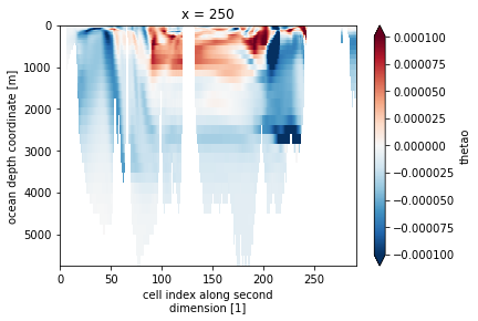
drift represents the slope of a linear regression at every grid point of the model. For demonstration purposes we will stick with the one grid point that we defined above. Lets first check if the trend seems right…
[24]:
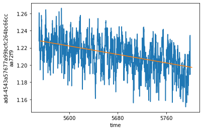
start = drift.trend_time_range.isel(bnds=0).data.tolist()
stop = drift.trend_time_range.isel(bnds=1).data.tolist()
time = xr.cftime_range(start, stop, freq='1MS')

# cut the control it to the time over which the trend was calculated
ds_control_cut = ds_control_rechunked.sel(time=slice(start, stop))

# use the linear slope from the same point to construct a trendline
trendline = xr.DataArray((np.arange(len(time)) * drift.thetao.isel(**roi).data) + ds_control_cut.thetao.isel(**roi, time=0).data, dims=['time'], coords={'time':time})
[28]:
ds_control_cut.thetao.isel(**roi).plot()
trendline.plot()
[28]:
[<matplotlib.lines.Line2D at 0x7f98bfa23460>]
Removing the drift from various datasets
We can remove this slope from either the control run
[29]:
control_detrended = remove_trend(ds_control, drift, 'thetao', ref_date=str(ds_control.time.data[0]))
control_detrended.isel(**roi).plot()
[29]:
[<matplotlib.lines.Line2D at 0x7f98b9de5490>]
Sure thats nice, but that’s not why we are here. Lets actually remove the trend from the control run from another run.
[30]:
ds_historical_dedrifted = remove_trend(ds_historical, drift, 'thetao', ref_date=str(ds_historical.time.data[0]))
ds_historical_dedrifted.isel(**roi).plot()
[30]:
[<matplotlib.lines.Line2D at 0x7f98bf89d040>]
[31]:
ds_historical_dedrifted
[31]:
<xarray.DataArray (time: 1980, lev: 45, y: 291, x: 360)>
dask.array<sub, shape=(1980, 45, 291, 360), dtype=float32, chunksize=(5, 45, 291, 360), chunktype=numpy.ndarray>
Coordinates:
  * time     (time) object 1850-01-16 12:00:00 ... 2014-12-16 12:00:00
  * x        (x) int32 0 1 2 3 4 5 6 7 8 ... 351 352 353 354 355 356 357 358 359
  * y        (y) int32 0 1 2 3 4 5 6 7 8 ... 282 283 284 285 286 287 288 289 290
    lat      (y, x) float64 dask.array<chunksize=(291, 360), meta=np.ndarray>
  * lev      (lev) float64 3.047 9.454 16.36 ... 5.126e+03 5.375e+03 5.625e+03
    lon      (y, x) float64 dask.array<chunksize=(291, 360), meta=np.ndarray>
Attributes:
    cell_measures:  area: areacello volume: volcello
    cell_methods:   area: mean where sea time: mean
    comment:        Diagnostic should be contributed even for models using co...
    long_name:      Sea Water Potential Temperature
    original_name:  votemper
    standard_name:  sea_water_potential_temperature
    units:          degC
drift_removed: linear_trend_CMIP.CCCma.CanESM5-CanOE.historical.r1i1p2f1...- time: 1980
- lev: 45
- y: 291
- x: 360
- dask.array<chunksize=(5, 45, 291, 360), meta=np.ndarray>
Array Chunk Bytes 34.77 GiB 89.92 MiB Shape (1980, 45, 291, 360) (5, 45, 291, 360) Count 2378 Tasks 396 Chunks Type float32 numpy.ndarray - time(time)object1850-01-16 12:00:00 ... 2014-12-...
- axis :
- T
- bounds :
- time_bnds
- long_name :
- time
- standard_name :
- time
array([cftime.DatetimeNoLeap(1850, 1, 16, 12, 0, 0, 0), cftime.DatetimeNoLeap(1850, 2, 15, 0, 0, 0, 0), cftime.DatetimeNoLeap(1850, 3, 16, 12, 0, 0, 0), ..., cftime.DatetimeNoLeap(2014, 10, 16, 12, 0, 0, 0), cftime.DatetimeNoLeap(2014, 11, 16, 0, 0, 0, 0), cftime.DatetimeNoLeap(2014, 12, 16, 12, 0, 0, 0)], dtype=object) - x(x)int320 1 2 3 4 5 ... 355 356 357 358 359
- long_name :
- cell index along first dimension
- units :
- 1
array([ 0, 1, 2, ..., 357, 358, 359], dtype=int32)
- y(y)int320 1 2 3 4 5 ... 286 287 288 289 290
- long_name :
- cell index along second dimension
- units :
- 1
array([ 0, 1, 2, ..., 288, 289, 290], dtype=int32)
- lat(y, x)float64dask.array<chunksize=(291, 360), meta=np.ndarray>
- bounds :
- vertices_latitude
- long_name :
- latitude
- standard_name :
- latitude
- units :
- degrees_north
Array Chunk Bytes 818.44 kiB 818.44 kiB Shape (291, 360) (291, 360) Count 7 Tasks 1 Chunks Type float64 numpy.ndarray - lev(lev)float643.047 9.454 ... 5.375e+03 5.625e+03
- axis :
- Z
- bounds :
- lev_bnds
- long_name :
- ocean depth coordinate
- positive :
- down
- standard_name :
- depth
- units :
- m
array([3.046773e+00, 9.454049e+00, 1.636397e+01, 2.389871e+01, 3.220929e+01, 4.148185e+01, 5.194513e+01, 6.387905e+01, 7.762451e+01, 9.359412e+01, 1.122835e+02, 1.342823e+02, 1.602840e+02, 1.910925e+02, 2.276233e+02, 2.708962e+02, 3.220169e+02, 3.821444e+02, 4.524429e+02, 5.340197e+02, 6.278525e+02, 7.347150e+02, 8.551112e+02, 9.892289e+02, 1.136922e+03, 1.297724e+03, 1.470893e+03, 1.655472e+03, 1.850365e+03, 2.054414e+03, 2.266454e+03, 2.485371e+03, 2.710133e+03, 2.939812e+03, 3.173588e+03, 3.410756e+03, 3.650712e+03, 3.892950e+03, 4.137047e+03, 4.382654e+03, 4.629485e+03, 4.877303e+03, 5.125919e+03, 5.375177e+03, 5.624952e+03]) - lon(y, x)float64dask.array<chunksize=(291, 360), meta=np.ndarray>
- bounds :
- vertices_longitude
- long_name :
- longitude
- standard_name :
- longitude
- units :
- degrees_east
Array Chunk Bytes 818.44 kiB 818.44 kiB Shape (291, 360) (291, 360) Count 10 Tasks 1 Chunks Type float64 numpy.ndarray
- cell_measures :
- area: areacello volume: volcello
- cell_methods :
- area: mean where sea time: mean
- comment :
- Diagnostic should be contributed even for models using conservative temperature as prognostic field.
- long_name :
- Sea Water Potential Temperature
- original_name :
- votemper
- standard_name :
- sea_water_potential_temperature
- units :
- degC
- drift_removed :
- linear_trend_CMIP.CCCma.CanESM5-CanOE.historical.r1i1p2f1.Omon.gn.v20190429_5550-01-16 12:00:00_5799-12-16 12:00:00
[32]:
ds_historical_dedrifted.attrs['drift_removed']
[32]:
'linear_trend_CMIP.CCCma.CanESM5-CanOE.historical.r1i1p2f1.Omon.gn.v20190429_5550-01-16 12:00:00_5799-12-16 12:00:00'
Note that the attributes now contain informations about the dataset and time frame over which the removed trend was computed!
[33]:
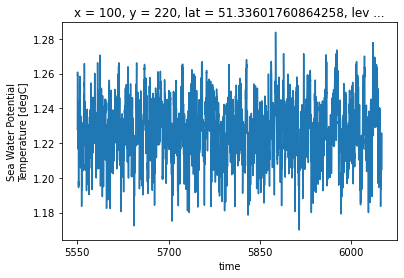
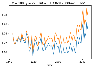
ds_historical.isel(**roi).thetao.coarsen(time=36).mean().plot()
ds_historical_dedrifted.isel(**roi).coarsen(time=36).mean().plot()
[33]:
[<matplotlib.lines.Line2D at 0x7f98eec61d60>]
You can also remove the trend from the ssp585 scenario in a way that is consistent with the historical run. The key here is the ref_date input. This should be set to the ‘branching’ timestep of the historical run for both experiments (which is 1850-01-01 for most CMIP6 historical experiments).
[36]:
ds_ssp585_dedrifted = remove_trend(
    ds_ssp585,
    drift,
    'thetao',
    ref_date=str(ds_historical.time.data[0])
    # Note that the ref_date is still the first time point of the *historical*run.
    # This ensures that the scenario is treated as an extension of the historical
    # run and the offset is calculated appropriately
)
[35]:
ds_historical.isel(**roi).thetao.coarsen(time=36, boundary='trim').mean().plot(color='C0', label='raw data')
ds_ssp585.isel(**roi).thetao.coarsen(time=36, boundary='trim').mean().plot(color='C0')
ds_historical_dedrifted.isel(**roi).coarsen(time=36, boundary='trim').mean().plot(color='C1', label='control drift removed')
ds_ssp585_dedrifted.isel(**roi).coarsen(time=36, boundary='trim').mean().plot(color='C1')
[35]:
[<matplotlib.lines.Line2D at 0x7f98ba0bd820>]
We are working on calculating the linear trends for common variables and store them in the cloud. Then you only have to apply
remove_trendand not the expensivecalculate_driftanymore. Stay tuned!
[ ]: